Fetching Sentinel-2 Imagery via STAC and AWS Open Data
As part of getting up to speed on Earth observation data pipelines, I wanted to go hands-on with actual satellite imagery before touching any model code. This note walks through how to query Sentinel-2 scenes using Element84’s STAC server and download a band directly from AWS Open Data.
What is STAC?
STAC (SpatioTemporal Asset Catalog) is a common specification for describing geospatial data. A catalog contains collections (datasets like Sentinel-2 L1C), and each collection contains items (individual scenes), each of which links to the actual files (assets), e.g., individual band GeoTIFFs.
Element84’s Earth Search is a publicly accessible STAC API that indexes satellite datasets hosted on AWS Open Data, including Sentinel-2.
Setup
from pystac_client import Client
import geopandas as gpd
from shapely.geometry import Polygon
import pandas as pd
import boto3
import os
import matplotlib.pyplot as plt
from osgeo import gdal
Connecting to the STAC Catalog
STAC_URL = "https://earth-search.aws.element84.com/v1"
catalog = Client.open(STAC_URL)

# List available collections
collections = [(c.id, c.title) for c in catalog.get_collections()]
print(collections)
A few notable collections in v1:
sentinel-2-l1c: Top-of-atmosphere reflectance (replacessentinel-s2-l2a-cogsfrom v0)sentinel-2-l2a: Surface reflectance with atmospheric correctioncop-dem-glo-30: Copernicus DEM
Note: The collection name changed between v0 and v1 of the Earth Search API. If you’re following older tutorials,
sentinel-s2-l2a-cogswill not work with the v1 endpoint.
Defining the Area of Interest and Search Parameters
# Area of interest: GeoJSON polygon (Sunnyvale, CA area)
aoi = {
    "coordinates": [[
        [-122.01047719743256, 37.3913836270592],
        [-122.01047719743256, 37.38072992443236],
        [-121.9932974844205,  37.38072992443236],
        [-121.9932974844205,  37.3913836270592],
        [-122.01047719743256, 37.3913836270592]
    ]],
    "type": "Polygon"
}

datefrom = "2025-07-01"
dateto   = "2025-07-31"
time_range = f"{datefrom}T00:00:00Z/{dateto}T23:59:59Z"

search = catalog.search(
    collections=["sentinel-2-l1c"],
    datetime=time_range,
    query={"eo:cloud_cover": {"lt": 50}},
    intersects=aoi,
    limit=500
)

items = list(search.items())
print(f"Found {len(items)} scenes.")
Inspecting the Results as a GeoDataFrame
Converting results to a GeoDataFrame makes it easy to inspect footprints and export to GeoJSON for visualization in QGIS or kepler.gl.
items_dict = search.get_all_items_as_dict()["features"]
items_df = pd.DataFrame(items_dict)

items_df['geometry'] = items_df['geometry'].apply(
    lambda x: Polygon(x['coordinates'][0])
)
items_gdf = gpd.GeoDataFrame(items_df, geometry='geometry', crs='EPSG:4326')

# Export scene footprints to GeoJSON
items_gdf[["id", "geometry"]].to_file('items.geojson', driver='GeoJSON')
Downloading a Band from S3
Rather than fetching over HTTPS, downloading via the S3 URI directly is faster and more reliable when you have AWS credentials configured.
# Collect RedEdge1 (Band 5, ~705nm) asset URLs
urls = [items_df['assets'][i]['rededge1']['href'] for i in range(len(items_df))]

# Convert HTTPS URL to S3 URI
target_url = urls[0]
s3_uri = target_url.replace(
    'https://sentinel-cogs.s3.us-west-2.amazonaws.com',
    's3://sentinel-cogs'
)

bucket_name = s3_uri.split('/')[2]
key = '/'.join(s3_uri.split('/')[3:])
local_path = os.path.join(os.getcwd(), key.split('/')[-1])

session = boto3.Session(profile_name='default')
session.resource('s3').Bucket(bucket_name).download_file(key, local_path)
print(f"Downloaded to: {local_path}")
The sentinel-cogs bucket is public and part of the AWS Open Data Registry, so no special permissions are needed; just valid AWS credentials for the request signing.
Displaying the Image
band5 = gdal.Open(local_path)
plt.imshow(band5.ReadAsArray())
plt.title("Sentinel-2 Band 5 (RedEdge1) — Sunnyvale, CA")
plt.colorbar()
plt.show()
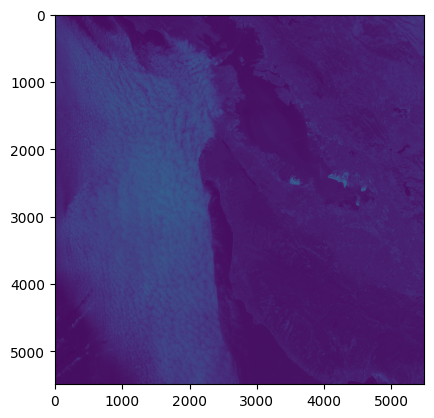
The image is ~5500×5500 pixels, covering a full Sentinel-2 tile (~55km × 55km at 20m resolution for Band 5). The San Francisco Bay is clearly visible on the right side.
Notes and Gotchas
- STAC API v0 vs v1: Collection names changed.
sentinel-s2-l2a-cogs(v0) →sentinel-2-l1c/sentinel-2-l2a(v1). Worth checking the Earth Search changelog if old code breaks. rasteriovsgdal:rasteriois a higher-level wrapper around GDAL and generally more convenient. It also supports streaming COGs directly from S3 without downloading first usingrasterio.open(s3_uri), worth trying next time to skip the local download step.- Default colormap:
plt.imshow()without a colormap argument uses viridis. For a more intuitive grayscale view of a single band, passcmap='gray'. - L1C vs L2A: L1C is top-of-atmosphere reflectance (raw); L2A has atmospheric correction applied and is more suitable for surface analysis. For most downstream ML tasks, L2A is the right choice.
Next Steps
- Try streaming the COG directly with
rasterioinstead of downloading - Create a true-color RGB composite from B04/B03/B02
- Look into
stackstacfor stacking multiple dates into an xarray