Quick recap of basic exploration strategy in RL - epsilon-greedy
Back to basics. I realized I had not written anything about reinforcement learning (RL) since I started this blog, despite having worked in RL for a while. I have been spending too much time with GANs lately :)
As with the previous post, this is part of my “reinventing-the-wheels” project to understand things deeply. Of course, it depends on your available time, but there are always benefits to implementing things yourself. You may discover how much impact a factor you had overlooked actually has, you may come up with new ideas as extensions while thinking things through, or you may simply build solid programming skills.
In this post, I will briefly review tabular Q-learning and \(\epsilon\)-greedy action selection, and list some advanced topics related to intrinsic reward and exploration.
Algorithms are implemented in reinventing-the-wheels/ML/rl/tabular_q.py
The problem
The target environment is FrozenLake-v0. (A larger version is also available: FrozenLake8x8-v0)
- The agent controls the movement of a character in a grid world
- Some tiles of the grid are walkable; others cause the agent to fall into the water
- The agent’s movement is stochastic (the ice is slippery), so the agent sometimes moves in an unintended direction, making the problem much more difficult despite its simple setup
- The agent is rewarded for finding a walkable path to the goal tile
- Reward is 1 if the agent reaches the goal, and 0 otherwise
- The episode ends when the agent reaches the goal or falls into a hole
The surface is described using a grid like the following:
    SFFF     S : starting point, safe
    FHFH     F : frozen surface, safe
    FFFH     H : hole, fall to your doom
    HFFG     G : goal, where the frisbee is located
Tabular Q-learning
Since the number of states in FrozenLake is small, the environment can be represented as a table. The agent learns the value of each state using the Q-learning algorithm (the full derivation is beyond the scope of this post).
To choose an action, the agent needs to estimate the value of each state and update those estimates based on experience. The simplest update rule is:
\[NewEstimate \leftarrow OldEstimate + StepSize [Target - OldEstimate]\]This simply says: “update your old estimate by an amount proportional to the error.”
The code looks like this (written step by step for clarity):
target = reward + GAMMA * np.max(self.values[next_state])
diff = target - self.values[curr_state][action]
self.values[curr_state][action] = self.values[curr_state][action] + ALPHA * diff
In the first line, you compute the sum of the reward just received and the discounted value of the next state. If your estimate is accurate, this quantity should equal the estimated value of the current state (Bellman equation), so the difference represents the error, as shown in the second line.
With the learning rule established, let’s move on.
\(\epsilon\)-greedy
One of the key challenges in RL is the explore–exploit tradeoff. For instance, the agent may know that stepping forward in state \(s\) yields a reward, but may be uncertain about what lies beyond. It can exploit its current knowledge and collect the known reward, but what if the path ahead leads to even greater rewards? Balancing exploration and exploitation is therefore critical. The simplest technique for encouraging exploration is the \(\epsilon\)-greedy algorithm.
1-1. Simple \(\epsilon\)-greedy
Below is a sample implementation. First, a random number is drawn and compared against a pre-specified value eps. If the random number is greater than eps, the agent exploits; otherwise, it explores.
def select_action_epsgreedy(self, state):
    """Return an action given the current state.
    Explore with probability of epsilon. When to exploit, action is determined greedily based on Q (state-action) value.
    Exploration probability is fixed.
    """
    # Generates a random value [0.0, 1.0) uniformly and perform greedy action selection if the value is greater than eps
    # Else, take a random action (= explore with probability eps)
    if random.random() > eps:
        action_values = self.values[state]
        max_value = np.max(action_values)
        idx = np.where(action_values == max_value)[0]
        if len(idx) > 1:
            # if multiple actions have the same high value, randomly pick one from those actions
            return np.random.choice(idx, 1)[0]
        else:
            return np.argmax(action_values)
    else:
        return env.action_space.sample()
1-2. Decaying \(\epsilon\)-greedy
Another variation is decaying \(\epsilon\)-greedy.
In the previous implementation, eps is fixed throughout training. It is more reasonable, however, to explore more at the early stages of learning and gradually shift toward exploitation.
To achieve this, we can use the following exponential decay schedule:
eps_start = 0.9
eps_end = 0.05
eps_decay = 200

eps = eps_end + (eps_start - eps_end) * math.exp(-1. * i / eps_decay)
This causes eps to decrease as shown below, with less exploration as training progresses.
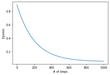
This makes intuitive sense: in the early stages, the agent knows little about the environment and needs to explore widely. Over time, through trial and error, the agent learns what works and can rely more on exploitation.
def select_action_decaying_epsgreedy(self, state, total_steps):
    """Return an action given the current state.
    Explore with probability epsilon. When to exploit, action is determined greedily based on Q (state-action) value.
    Exploration probability is decaying as more steps are taken.
    """
    # Generates a random value [0.0, 1.0) uniformly and perform greedy action selection if the value is greater than eps
    # Else, take a random action (= explore with probability eps)
    eps = eps_end + (eps_start - eps_end) * math.exp(-1. * self.total_steps / eps_decay)
    if random.random() > eps:
        action_values = self.values[state]
        max_value = np.max(action_values)
        idx = np.where(action_values == max_value)[0]
        if len(idx) > 1:
            # if multiple actions have the same high value, randomly pick one from those actions
            return np.random.choice(idx, 1)[0]
        else:
            return np.argmax(action_values)
    else:
        return self.env.action_space.sample()
This \(\epsilon\)-greedy exploration strategy is used in DeepMind’s seminal paper showing that a Deep Q-learning agent can achieve superhuman performance on Atari games.
One downside is that the decay hyperparameter eps_decay requires tuning, which can be tedious.
Experiments
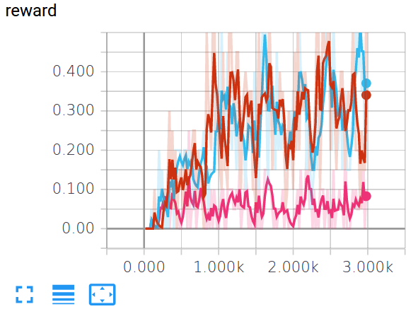
The figure below compares a simple greedy agent (pink), \(\epsilon\)-greedy (red), and \(\epsilon\)-greedy with decay (blue).
Since reward is either 0 or 1 in FrozenLake and individual episode results are noisy, the values shown are averages over every 20 epochs. Both \(\epsilon\)-greedy variants outperform the simple greedy strategy.
Note: the environment has stochasticity due to the slippery floor. Setting is_slippery=False makes the problem considerably easier and results in a much sharper performance increase.
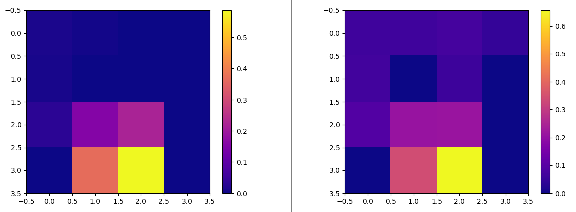
One more experiment. The heatmap below shows Q values after training for the greedy agent (left) and the \(\epsilon\)-greedy agent (right). The right figure shows that the \(\epsilon\)-greedy agent visited more cells; note the higher values in the upper portion of the grid.
Going further
Simple extensions: Adding noise to weights or observations
Some research suggests that simply adding noise to a neural network’s parameters can effectively encourage exploration:
Uncertainty measures
Although \(\epsilon\)-greedy action selection encourages exploration of non-greedy actions, it provides no notion of how promising those non-greedy actions are relative to each other. Upper Confidence Bound (UCB) addresses this by explicitly modeling uncertainty:
\[A_t = argmax_a \Big[ Q_t(a) + c \sqrt{\frac{\ln t}{N_t(a)}} \Big]\]\(N_t(a)\) denotes the number of times action \(a\) has been selected prior to time \(t\). The square root term acts as an uncertainty measure: the more frequently action \(a\) has been taken, the smaller the term (i.e., more certainty). The logarithm in the numerator ensures that this uncertainty grows relatively slowly over time.
Intrinsic reward, curiosity, and surprise
Exploration is a particularly interesting problem when rewards are sparse. If an agent rarely receives any reward signal, it has no way to update its value estimates and cannot determine what to do. In such cases, intrinsic reward (also called “curiosity”) can help.
The basic idea is to reward an agent for visiting unexplored states. “Curiosity” is an apt name: the agent is rewarded for satisfying its internal curiosity by experiencing new states (e.g., visiting unexplored areas of a maze).
Although this post only covers basic exploration strategies, there are many interesting ideas on this topic. I maintain a GitHub repository of paper summaries with notes on some of the topics above, if you are interested.
Whenever I step back and reflect on what we are trying to reverse-engineer, I feel humbled and amazed at how children naturally begin exploring, and how humans instinctively balance exploration and exploitation throughout their lives. So many things are still waiting to be discovered. Keep exploring!